Unlocking TPU Performance with Custom MatMul Kernels using JAX Pallas

Matrix multiplication (MatMul) sits at the heart of machine learning. Efficient implementation is crucial, especially when working with hardware accelerators like Google’s TPUs. JAX’s Pallas framework empowers developers to write low-level, highly optimized kernels tailored specifically for TPUs. In this post, I’ll share my preliminary exploration of MatMul kernel implementations using JAX Pallas, highlighting how different optimizations impact performance on TPUs.

Why Optimize MatMul for TPUs?

TPUs, unlike GPUs, utilize SIMD systolic arrays designed for highly parallel computations in machine learning workloads. However, optimizing performance requires careful consideration of memory usage, parallelization strategy, and data precision.

Let’s dive into different implementations and the insights they provide.

Kernel Implementations Explored

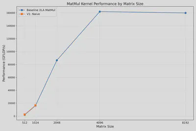
Kernel 1. Naive MatMul

This straightforward kernel loads entire matrices into TPU’s vector memory (VMEM):

def matmul_v1_kernel(a_ref, b_ref, o_ref):
  o_ref[...] = a_ref[...] @ b_ref[...]

With o_ref[...] = a_ref[...] @ b_ref[...], the input matrices [M, K], [K, N] are loaded into VMEM, and the output matrix [M, N] is stored in the VMEM While simple, it quickly runs out of memory for large matrices (>1024), highlighting the need for smarter strategies. It resulted in a high memory usage. As shown in the figure below, it can only process M=K=N <= 1024 sizes. For [2048, 2048] @ [2048, 2048] = [2048, 2048], we got overflow error “Failed: RESOURCE_EXHAUSTED: Ran out of memory in memory space vmem…”.

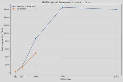
Kernel 2. Parallel MatMul

Splitting matrices into smaller chunks reduces VMEM usage:

def matmul_v2_parallel_kernel(a_ref, b_ref, o_ref):
  o_ref[...] = a_ref[...] @ b_ref[...]

@functools.partial(jax.jit, static_argnames=['N'])
def run_matmul_v2(a: jax.Array, b: jax.Array, N: int):
  kernel = pl.pallas_call(
      matmul_v2_parallel_kernel,
      grid=(N, N),
      in_specs=[
          pl.BlockSpec((a.shape[0] // N, a.shape[1]), lambda i, j: (i, 0)),
          pl.BlockSpec((b.shape[0], b.shape[1] // N), lambda i, j: (0, j)),
      ],
      out_specs=pl.BlockSpec(
        (a.shape[0] // N, b.shape[1] // N), lambda i, j: (i, j)),
      out_shape=jax.ShapeDtypeStruct((a.shape[0], b.shape[1]), a.dtype)
  )
  return kernel(a, b)

This kernel splits matrix A by rows and B by columns. Although it reduces memory usage, the achieved parallelism still lags behind XLA’s built-in jnp.matmul(). It improves the memory usage slightly. The figure below shows the results for N=4 parallelism. We can calculate M=K=N <= 2048 sizes now. However, we also find the performance is not as good as XLA library jnp.matmul().

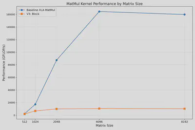
Kernel 3. Block-Based MatMul (3D Grid)

Employing a 3D grid approach further refines memory management: Previously the input matrices of size [block, M] or [M, block] are still loaded into VMEM. One straightforward thought is to implement block-based matmul using a 3D grid, rather than the row/column split. We can define [‘bm’, ‘bk’, ‘bn’] to split the input and output matrices. In the kernel code, we need to initialize the o_ref[...] for each iteration of K.

def matmul_v3_block_kernel(a_ref, b_ref, o_ref):
  @pl.when(pl.program_id(2) == 0)
  def init():
    o_ref[...] = jnp.zeros_like(o_ref)
  # Accumulates the multiplication for this block.
  o_ref[...] += a_ref[...] @ b_ref[...]


@functools.partial(jax.jit, static_argnames=['bm', 'bk', 'bn'])
def run_matmul_v3(
    a: jax.Array,
    b: jax.Array,
    *,
    bm: int = 128,
    bk: int = 128,
        bn: int = 128):

  m, k = a.shape
  _, n = b.shape
  assert k == b.shape[0]

  run_kernel = pl.pallas_call(
      matmul_v3_block_kernel,
      grid=(m // bm, n // bn, k // bk),
      in_specs=[
          pl.BlockSpec((bm, bk), lambda i, j, k: (i, k)),
          pl.BlockSpec((bk, bn), lambda i, j, k: (k, j)),
      ],
      out_specs=pl.BlockSpec((bm, bn), lambda i, j, k: (i, j)),
      out_shape=jax.ShapeDtypeStruct((m, n), a.dtype),
  )
  return run_kernel(a, b)

This implementation significantly reduces memory overhead and successfully handles larger matrices, but still does not match the performance of optimized libraries. The figure below shows the successful runs for all sizes, with relatively bad performance compared to XLA library jnp.matmul().

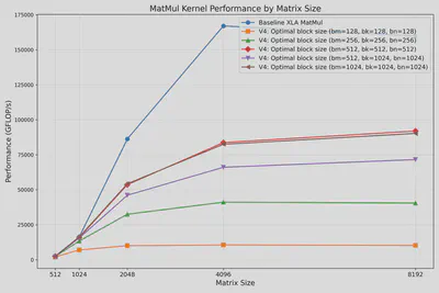
Kernel 4. Optimal Block Size Strategy

TPUs are different from GPUs. When writing CUDA kernels, users need to think about the accesses from the view of threads which happen in parallel to each other However, TPUs are actually a SIMD systolic array device, each kernel could be viewed as sequential execution.

Thus, we may search for the optimal block sizes for the best performance, because the loaded LHS can be reused for adjacent calculations.

The figure below shows a search for the best block size. It can be found that (bm, bk, bn) == (512, 512, 512) gives the best FLOP/s for this setting.

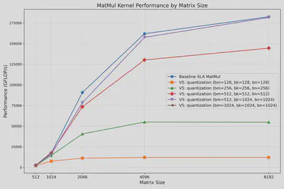
Kernel 5. Precision Optimization: Quantization

The optimal block sizes can change for different configs, including the precisions being used. The figure below shows the best performance for dtype = BFLOAT16, where (bm, bk, bn) == (512, 1024, 1024) almost achieves the performance of XLA library jnp.matmul().

Key Insights

• Memory Management: Effective memory splitting and block management are critical to leverage TPU parallelism.
• Block Sizing: Optimal block size selection significantly influences performance, necessitating empirical tuning.
• Precision Matters: Using lower precision formats like BFLOAT16 improves performance and memory efficiency, especially at scale.

Through this exploration using JAX’s Pallas framework, we’ve uncovered valuable insights into TPU optimization strategies. Custom kernel development allows developers to push hardware capabilities further, achieving significant performance gains essential for accelerating ML workloads.

Check out the repository to replicate and explore further!

Acknowledgements

This project is inspired by JAX’s Pallas framework and builds upon the TPU programming model.